Large Eddy Simulation

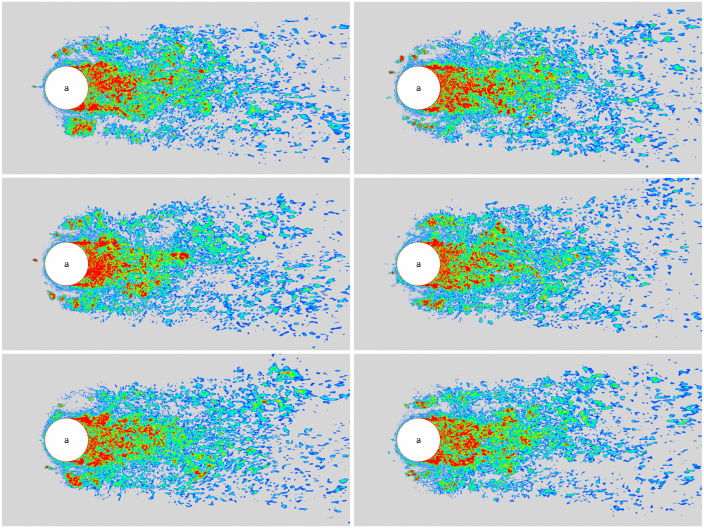
Resolving eddies (vortices) of all sizes in a turbulent flow is prohibitively expensive. Instead, we can just resolve the large eddies, but model the effects of the small ones in order to reduce the computational cost. This is the fundamental idea behind large eddy simulation.

To model the small eddies, we need to perform a spatial filtering on the original flow equations. The spatial filtering on any variable $f$ can be written in the following form, $$ \bar{f}(x) = \int_{\Omega}G(x-x')f(x')dx', $$ where $\bar{f}$ is the filtered variable, $G(x)$ is the kernel of the filter, $\Omega$ is the size of the filer (which is usually taken as mesh size). For compressible flow equations, in addition to the above filter, the following Favre filter makes the filtered equations simpler, $$ \widetilde{f} = \frac{\overline{\rho f}}{\bar{\rho}}, $$ where $\widetilde{f}$ is a Favre-filtered variable, and $\rho$ is density. Applying these filters to the flow equations, we will get $$ \begin{aligned} &\frac{\partial\bar{\rho}}{\partial t} + \frac{\partial\bar{\rho}\widetilde{u}_j}{\partial x_j} = 0, \\[1em] &\frac{\partial\bar{\rho}\widetilde{u}_i}{\partial t} + \frac{\partial}{\partial x_j}(\bar{\rho}\widetilde{u}_i\widetilde{u}_j+\bar{p}\delta_{ij}) = \frac{\partial\widetilde{\tau}_{ij}}{\partial x_j} - \frac{\partial\tau^{SGS}_{ij}}{\partial x_j},\\[1em] &\frac{\partial\bar{\rho}\widetilde{E}}{\partial t} + \frac{\partial}{\partial x_j}\Big((\bar{\rho}\widetilde{E}+\bar{p})\widetilde{u}_j\Big) = \frac{\partial}{\partial x_j}(\widetilde{u}_i\widetilde{\tau}_{ij}) - \frac{\partial\bar{q}_j}{\partial x_j} - \frac{\partial q^{SGS}_j}{\partial x_j}, \end{aligned} $$ where $\tau_{ij}^{SGS}$ and $q_j^{SGS}$ are the subgrid-scale (SGS) stress tensor and heat flux vector with the following expressions: $$ \begin{aligned} \tau_{ij}^{SGS} &= \bar{\rho}(\widetilde{u_i u_j} - \widetilde{u}_i\widetilde{u}_j), \\[1.0em] q_j^{SGS} &= \bar{\rho}(\widetilde{u_jT} - \widetilde{u}_j\widetilde{T}). \end{aligned} $$ These two terms are modeled using SGS models. For example, the following Smagorinsky model (assume equilibrium energy production and dissipation in small scales), $$ \begin{aligned} \tau_{ij}^{SGS} - \dfrac{1}{3} \tau_{kk}^{SGS} \delta_{ij} &= -2 \bar{\rho} \nu_t (\widetilde{S}_{ij} - \dfrac{1}{3} \widetilde{S}_{kk} \delta_{ij} ) , \\[1.0em] q_j^{SGS} &= -\dfrac{\bar{\rho} \nu_t}{Pr_t} \dfrac{\partial \widetilde{T}}{\partial x_j}, \end{aligned} $$ where $$ \widetilde{S}_{ij}= \dfrac{1}{2} \left(\dfrac{\partial \widetilde{u}_i}{\partial x_j} + \dfrac{\partial \widetilde{u}_j}{\partial x_i} \right), \\[1em] \nu_t = (C_s \Delta)^2 \sqrt{2 \widetilde{S}_{ij} \widetilde{S}_{ij}} = (C_s \Delta)^2 \vert\widetilde{S}\vert, $$ are the strain-rate tensor and the turbulent eddy viscosity, respectively; $Pr_t$ is the turbulent Prandtl number whose value is in the range $[0.3,0.9]$; $C_s$ is an empirical constant; $\Delta$ represents grid size.