Flux Reconstruction Method

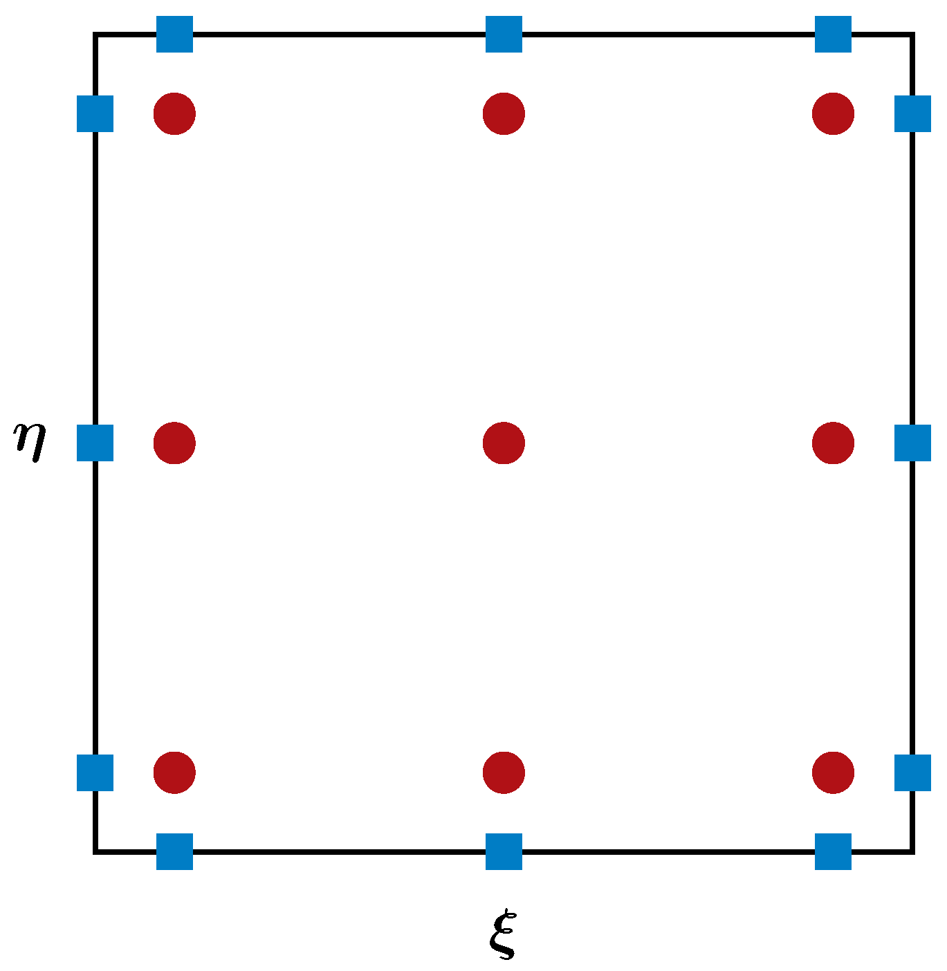
The FR method further improves the efficiency of the SD method by collocating the SPs and FPs in the interior of a computational element. The figure below sketches the distribution of the SPs (red dots) and FPs (bondary blue dots) for a third-order FR method. Similar to the SD method, the solution and flux polynomials are constructed using tensor products of the interpolation bases, $\begin{aligned} \widetilde{\mathbf{Q}}(\xi,\eta) &= \sum_{j=1}^{N} \sum_{i=1}^{N} \widetilde{\mathbf{Q}}_{i,j} h_i(\xi) h_j(\eta), \\ \widetilde{\mathbf{F}}(\xi,\eta) &= \sum_{j=1}^{N} \sum_{i=1}^{N} \widetilde{\mathbf{F}}_{i,j} h_i(\xi) h_j(\eta), \\ \widetilde{\mathbf{G}}(\xi,\eta) &= \sum_{j=1}^{N} \sum_{i=1}^{N} \widetilde{\mathbf{G}}_{i,j} h_i(\xi) h_j(\eta). \end{aligned}$ Due to the first-order spatial derivatives on the flux terms in the Navier-Stokes equations, the flux polynomials need to be at least one-degree higher than the solution polynomials to give the correct orders of accuracy. To achieve this goal, the above flux polynomials are reconstructed using higher-degree correction polynomials. For example, the reconstructed (corrected) flux polynomial in the $\xi$-direction is, $\widehat{\mathbf{F}}(\xi) = \widetilde{\mathbf{F}}(\xi) + (\widetilde{\mathbf{F}}_L^{com} - \widetilde{\mathbf{F}}_L) \cdot g_L(\xi) + (\widetilde{\mathbf{F}}_R^{com} - \widetilde{\mathbf{F}}_R) \cdot g_R(\xi),$ where $\widetilde{\mathbf{F}}$ is the original flux, $\widetilde{\mathbf{F}}_L^{com}$ and $\widetilde{\mathbf{F}}_R^{com}$ are the common fluxes on the left and the right boundaries, $\widetilde{\mathbf{F}}_L$ and $\widetilde{\mathbf{F}}_R$ are the original discontinuous boundary fluxes, $g_L$ and $g_R$ are the left and the right correction polynomials. The correction functions must satisfy the following conditions to ensure continuity, $g_L(0) = 1, \quad g_L(1) = 0; \quad g_R(0) = 0, \quad g_R(1) = 1.$ The user can define extra conditions to construct a correction polynomial. Once the fluxes are reconstructed, the remaining steps are essentially identical to those of the SD method.