Arbitrary Lagrangian-Eulerian Method

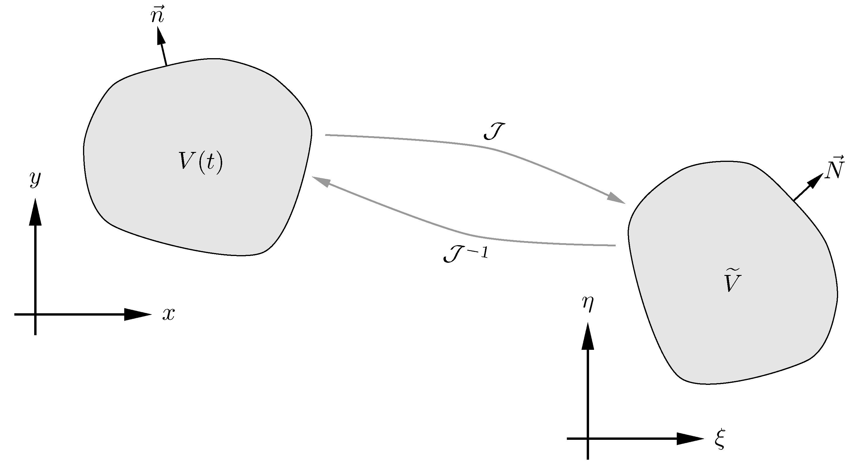
The ALE method is ideal for dealing with moving meshes by mapping them to a fixed reference space in which the governing equations are solved. The figure below shows a moving mesh for a plunging and pitching airfoil and a schematic of the mapping.

Assume a moving domain $V(t)$ is mapped from the physical time and space $(t,x,y)$ to a fixed domain $\widetilde{V}$ in the computational time and space $(\tau,\xi,\eta)$, where $\tau=t$ is time. It can be shown that the Navier-Stokes equations will take the following conservative form in the computational space, $\frac{\partial \widetilde{\mathbf{Q}}} {\partial t} + \frac{\partial \widetilde{\mathbf{F}}} {\partial \xi} + \frac{\partial \widetilde{\mathbf{G}}} {\partial \eta} = 0,$ where the computational variable and fluxes are related to the physical ones through $\left( \begin{array}{c} \widetilde{\mathbf{Q}} \\ \widetilde{\mathbf{F}} \\ \widetilde{\mathbf{G}} \end{array} \right) = |\mathcal{J}|\mathcal{J}^{-1} \left( \begin{array}{c} \mathbf{Q} \\ \mathbf{F} \\ \mathbf{G} \end{array} \right),$ where $|\mathcal{J}| = \left| \frac{\partial(t,x,y)}{\partial(\tau,\xi,\eta)} \right| = \left| \begin{matrix} 1 & 0 & 0 \\ x_t & x_{\xi} & x_{\eta} \\ y_t & y_{\xi} & y_{\eta} \end{matrix} \right|,$ $\mathcal{J}^{-1} = \frac{\partial(\tau,\xi,\eta)}{\partial(t,x,y)} = \frac{1}{|\mathcal{J}|} \begin{bmatrix} \phantom{-} |\mathcal{J}| & \phantom{-}0 & \phantom{-}0 \\ -x_t y_\eta + y_t x_\eta & \phantom{-}y_\eta & -x_\eta \\ \phantom{-}x_t y_\xi - y_t x_\xi & -y_\xi & \phantom{-} x_\xi \end{bmatrix}.$ The above derivation is in a general form. Alternatively, the ALE method can be cast into a two-step procedure. In the first step, the physical fluxes are modified to take into account grid velocities as, $\mathbf{F}^\prime = \mathbf{F} - u_g \mathbf{Q}, ~ \mathbf{G}^\prime = \mathbf{G} - v_g \mathbf{Q},$ where $(u_g,v_g)=(x_t,y_t)$ are the grid velocities, $\mathbf{F}$ and $\mathbf{G}$ are the original physical fluxes. In the second step, the modified fluxes are transformed to the computational ones (i.e., $\widetilde{\mathbf{F}}$ and $\widetilde{\mathbf{G}}$) in the same way as for fixed grids (see the SD method for details).